I joined AWS in 2021, and since then I’ve watched the Amazon Elastic Compute Cloud (Amazon EC2) instance family grow at a pace that still surprises me. From AWS Graviton-powered instances to specialized accelerated computing options, it feels like every few months there’s a new instance type landing that pushes performance boundaries further. As of February 2026, AWS offers over 1,160 Amazon EC2 instance types, and that number keeps climbing.
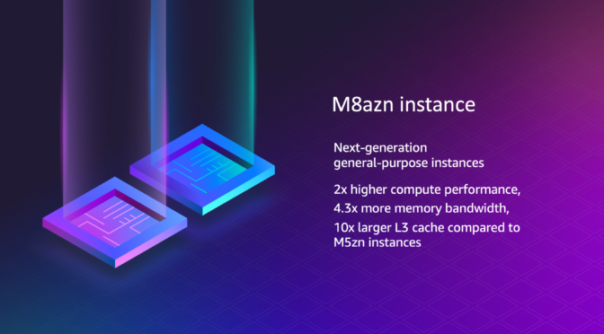
This week’s opening news is a good example: The general availability of Amazon EC2 M8azn instances. These are general purpose, high-frequency, high-network instances powered by fifth generation AMD EPYC processors, offering the highest maximum CPU frequency in the cloud at 5 GHz. Compared to the previous generation M5zn instances, M8azn instances deliver up to 2x compute performance, 4.3x higher memory bandwidth, and a 10x larger L3 cache. They also provide up to 2x networking throughput and up to 3x Amazon Elastic Block Store (Amazon EBS) throughput compared with M5zn.

Built on the AWS Nitro System using sixth generation Nitro Cards, M8azn instances target workloads such as real-time financial analytics, high-performance computing, high-frequency trading, CI/CD pipelines, gaming, and simulation modeling across automotive, aerospace, energy, and telecommunications. The instances feature a 4:1 ratio of memory to vCPU and are available in 9 sizes ranging from 2 to 96 vCPUs with up to 384 GiB of memory, including two bare metal variants. For more information visit the Amazon EC2 M8azn instance page.
Last week’s launches
Here are some of the other announcements from last week:
- Amazon Bedrock adds support for six fully managed open weights models – Amazon Bedrock now supports DeepSeek V3.2, MiniMax M2.1, GLM 4.7, GLM 4.7 Flash, Kimi K2.5, and Qwen3 Coder Next. These models span frontier reasoning and agentic coding workloads. DeepSeek V3.2 and Kimi K2.5 target reasoning and agentic intelligence, GLM 4.7 and MiniMax M2.1 support autonomous coding with large output windows, and Qwen3 Coder Next and GLM 4.7 Flash provide cost-efficient alternatives for production deployment. These models are powered by Project Mantle and provide out-of-the-box compatibility with OpenAI API specifications. With the launch, you can also use new open weight models–DeepSeek v3.2 , MiniMax 2.1, and Qwen3 Coder Next in Kiro, a spec-driven AI development tool.
- Amazon Bedrock expands support for AWS PrivateLink – Amazon Bedrock now supports AWS PrivateLink for the
bedrock-mantleendpoint, in addition to existing support for thebedrock-runtimeendpoint. The bedrock-mantle endpoint is powered by Project Mantle, a distributed inference engine for large-scale machine learning model serving on Amazon Bedrock. Project Mantle provides serverless inference with quality of service controls, higher default customer quotas with automated capacity management, and out-of-the-box compatibility with OpenAI API specifications. AWS PrivateLink support for OpenAI API-compatible endpoints is available in 14 AWS Regions. To get started, visit the Amazon Bedrock console or the OpenAI API compatibility documentation. - Amazon EKS Auto Mode announces enhanced logging for managed Kubernetes capabilities – You can now configure log delivery sources using Amazon CloudWatch Vended Logs in Amazon EKS Auto Mode. This helps you collect logs from Auto Mode’s managed Kubernetes capabilities for compute autoscaling, block storage, load balancing, and pod networking. Each Auto Mode capability can be configured as a CloudWatch Vended Logs delivery source with built-in AWS authentication and authorization at a reduced price compared to standard CloudWatch Logs. You can deliver logs to CloudWatch Logs, Amazon S3, or Amazon Data Firehose destinations. This feature is available in all Regions where EKS Auto Mode is available.
- Amazon OpenSearch Serverless now supports Collection Groups – You can use new Collection Groups to share OpenSearch Compute Units (OCUs) across collections with different AWS Key Management Service (AWS KMS) keys. Collection Groups reduce overall OCU costs through a shared compute model while maintaining collection-level security and access controls. They also introduce the ability to specify minimum OCU allocations alongside maximum OCU limits, providing guaranteed baseline capacity at startup for latency-sensitive applications. Collection Groups are available in all Regions where Amazon OpenSearch Serverless is currently available.
- Amazon RDS now supports backup configuration when restoring snapshots – You can view and modify the backup retention period and preferred backup window before and during snapshot restore operations. Previously, restored database instances and clusters inherited backup parameter values from snapshot metadata and could only be modified after restore was complete. You can now view backup settings as part of automated backups and snapshots, and specify or modify these values when restoring, eliminating the need for post-restoration modifications. This is available for all Amazon RDS database engines (MySQL, PostgreSQL, MariaDB, Oracle, SQL Server, and Db2) and Amazon Aurora (MySQL-Compatible and PostgreSQL-Compatible editions) in all AWS commercial Regions and AWS GovCloud (US) Regions at no additional cost.
For a full list of AWS announcements, be sure to keep an eye on the What’s New with AWS page.
Upcoming AWS events
Check your calendar and sign up for upcoming AWS events:
AWS Summits – Join AWS Summits in 2026, free in-person events where you can explore emerging cloud and AI technologies, learn best practices, and network with industry peers and experts. Upcoming Summits include Paris (April 1), London (April 22), and Bengaluru (April 23–24).
AWS AI and Data Conference 2026 – A free, single-day in-person event on March 12 at the Lyrath Convention Centre in Ireland. The conference covers designing, training, and deploying agents with Amazon Bedrock, Amazon SageMaker, and QuickSight, integrating them with AWS data services, and applying governance practices to operate them at scale. The agenda includes strategic guidance and hands-on labs for architects, developers, and business leaders.
AWS Community Days – Community-led conferences where content is planned, sourced, and delivered by community leaders, featuring technical discussions, workshops, and hands-on labs. Upcoming events include Ahmedabad (February 28), Slovakia (March 11), and Pune (March 21).
Join the AWS Builder Center to connect with builders, share solutions, and access content that supports your development. Browse here for upcoming AWS led in-person and virtual events and developer-focused events.
That’s all for this week. Check back next Monday for another Weekly Roundup!
This post is part of our Weekly Roundup series. Check back each week for a quick roundup of interesting news and announcements from AWS!