This
post was originally published on
this siteTwenty years ago today, on March 14, 2006, Amazon Simple Storage Service (Amazon S3) quietly launched with a modest one-paragraph announcement on the What’s New page:
Amazon S3 is storage for the Internet. It is designed to make web-scale computing easier for developers. Amazon S3 provides a simple web services interface that can be used to store and retrieve any amount of data, at any time, from anywhere on the web. It gives any developer access to the same highly scalable, reliable, fast, inexpensive data storage infrastructure that Amazon uses to run its own global network of web sites.
Even Jeff Barr’s blog post was only a few paragraphs, written before catching a plane to a developer event in California. No code examples. No demo. Very low fanfare. Nobody knew at the time that this launch would shape our entire industry.
The early days: Building blocks that just work
At its core, S3 introduced two straightforward primitives: PUT to store an object and GET to retrieve it later. But the real innovation was the philosophy behind it: create building blocks that handle the undifferentiated heavy lifting, which freed developers to focus on higher-level work.
From day one, S3 was guided by five fundamentals that remain unchanged today.
Security means your data is protected by default. Durability is designed for 11 nines (99.999999999%), and we operate S3 to be lossless. Availability is designed into every layer, with the assumption that failure is always present and must be handled. Performance is optimized to store virtually any amount of data without degradation. Elasticity means the system automatically grows and shrinks as you add and remove data, with no manual intervention required.
When we get these things right, the service becomes so straightforward that most of you never have to think about how complex these concepts are.
S3 today: Scale beyond imagination
Throughout 20 years, S3 has remained committed to its core fundamentals even as it’s grown to a scale that’s hard to comprehend.
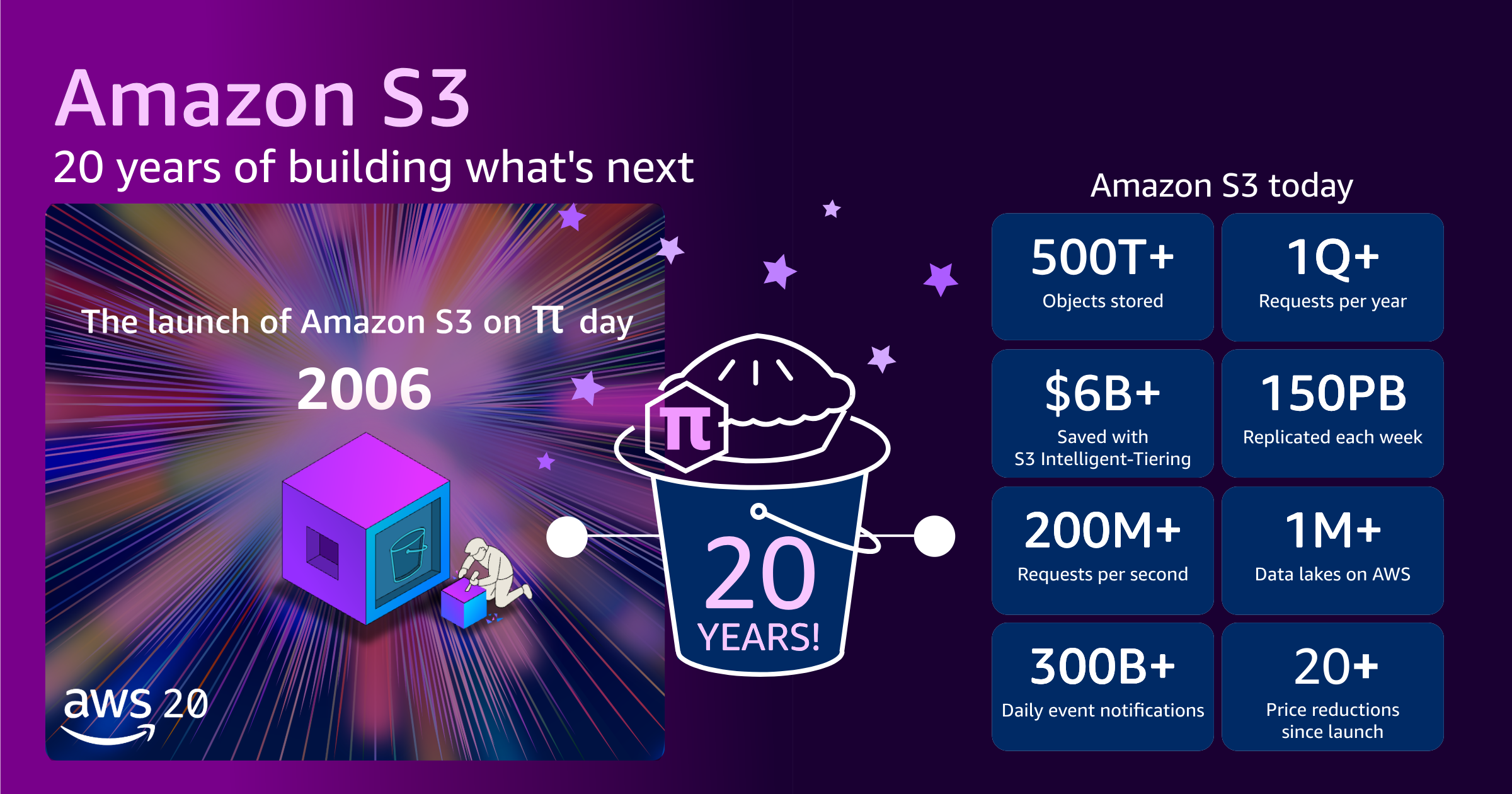
When S3 first launched, it offered approximately one petabyte of total storage capacity across about 400 storage nodes in 15 racks spanning three data centers, with 15 Gbps of total bandwidth. We designed the system to store tens of billions of objects, with a maximum object size of 5 GB. The initial price was 15 cents per gigabyte.

Today, S3 stores more than 500 trillion objects and serves more than 200 million requests per second globally across hundreds of exabytes of data in 123 Availability Zones in 39 AWS Regions, for millions of customers. The maximum object size has grown from 5 GB to 50 TB, a 10,000 fold increase. If you stacked all of the tens of millions S3 hard drives on top of each other, they would reach the International Space Station and almost back.
Even as S3 has grown to support this incredible scale, the price you pay has dropped. Today, AWS charges slightly over 2 cents per gigabyte. That’s a price reduction of approximately 85% since launch in 2006. In parallel, we’ve continued to introduce ways to further optimize storage spend with storage tiers. For example, our customers have collectively saved more than $6 billion in storage costs by using Amazon S3 Intelligent-Tiering as compared to Amazon S3 Standard.
Over the past two decades, the S3 API has been adopted and used as a reference point across the storage industry. Multiple vendors now offer S3 compatible storage tools and systems, implementing the same API patterns and conventions. This means skills and tools developed for S3 often transfer to other storage systems, making the broader storage landscape more accessible.
Despite all of this growth and industry adoption, perhaps the most remarkable achievement is this: the code you wrote for S3 in 2006 still works today, unchanged. Your data went through 20 years of innovation and technical advances. We migrated the infrastructure through multiple generations of disks and storage systems. All the code to handle a request has been rewritten. But the data you stored 20 years ago is still available today, and we’ve maintained complete API backward compatibility. That’s our commitment to delivering a service that continually “just works.”
The engineering behind the scale
What makes S3 possible at this scale? Continuous innovation in engineering.
Much of what follows is drawn from a conversation between Mai-Lan Tomsen Bukovec, VP of Data and Analytics at AWS, and Gergely Orosz of The Pragmatic Engineer. The in-depth interview goes further into the technical details for those who want to go deeper. In the following paragraphs, I share some examples:
At the heart of S3 durability is a system of microservices that continuously inspect every single byte across the entire fleet. These auditor services examine data and automatically trigger repair systems the moment they detect signs of degradation. S3 is designed to be lossless: the 11 nines design goal reflects how the replication factor and re-replication fleet are sized, but the system is built so that objects aren’t lost.
S3 engineers use formal methods and automated reasoning in production to mathematically prove correctness. When engineers check in code to the index subsystem, automated proofs verify that consistency hasn’t regressed. This same approach proves correctness in cross-Region replication or for access policies.
Over the past 8 years, AWS has been progressively rewriting performance-critical code in the S3 request path in Rust. Blob movement and disk storage have been rewritten, and work is actively ongoing across other components. Beyond raw performance, Rust’s type system and memory safety guarantees eliminate entire classes of bugs at compile time. This is an essential property when operating at S3 scale and correctness requirements.
S3 is built on a design philosophy: “Scale is to your advantage.” Engineers design systems so that increased scale improves attributes for all users. The larger S3 gets, the more de-correlated workloads become, which improves reliability for everyone.
Looking forward
The vision for S3 extends beyond being a storage service to becoming the universal foundation for all data and AI workloads. Our vision is simple: you store any type of data one time in S3, and you work with it directly, without moving data between specialized systems. This approach reduces costs, eliminates complexity, and removes the need for multiple copies of the same data.
Here are a few standout launches from recent years:
- S3 Tables – Fully managed Apache Iceberg tables with automated maintenance that optimize query efficiency and reduce storage cost over time.
- S3 Vectors – Native vector storage for semantic search and RAG, supporting up to 2 billion vectors per index with sub-100ms query latency. In only 5 months (July–December 2025), you created more than 250,000 indices, ingested more than 40 billion vectors, and performed more than 1 billion queries.
- S3 Metadata – Centralized metadata for instant data discovery, removing the need to recursively list large buckets for cataloging and significantly reducing time-to-insight for large data lakes.
Each of these capabilities operates at S3 cost structure. You can handle multiple data types that traditionally required expensive databases or specialized systems but are now economically feasible at scale.
From 1 petabyte to hundreds of exabytes. From 15 cents to 2 cents per gigabyte. From simple object storage to the foundation for AI and analytics. Through it all, our five fundamentals–security, durability, availability, performance, and elasticity–remain unchanged, and your code from 2006 still works today.
Here’s to the next 20 years of innovation on Amazon S3.
— seb

 Community Hero Maurizio is a CTO and organizer of the AWS User Group Basilicata, recognized for his dedication to building tech ecosystems where they previously did not exist. For over a decade, he has pioneered cloud culture through a philosophy centered on genuine human connection and knowledge transfer. He founded an international tech conference in a small mountain village, creating a unique space where global experts and local talent meet, blending deep technical sessions on cloud architectures, DevOps, and web scaling with unconventional networking experiences. Beyond organizing events, Maurizio is a tireless mentor working across generations, which span from introducing children to coding to helping university students and professionals transition into cloud architecture. His impact is defined by a rare combination of technical leadership and inclusive community building that draws people from across Europe.
 Artificial Intelligence Hero Ray Goh is a seasoned AWS machine learning and AI community leader based in Singapore and a long-standing contributor in various AWS community programs since 2018, from AWS ASEAN Cloud Warrior and AWS Dev/Cloud Alliance to being part of the pioneer batch of AWS Community Builders in 2020. He founded The Gen-C (a Generative AI Learning Community) in 2024, organizing regular public workshops at libraries across Singapore on topics ranging from LLM fine-tuning to AI agents on AWS. Ray has spoken at AWS re:Invent, AWS Summit ASEAN, AWS Community Day Hong Kong, and numerous user group meetups, and guest-authored for the AWS Machine Learning Blog. He spearheaded the world’s largest enterprise AWS DeepRacer program for DBS Bank in 2020, upskilling over 3,100 employees, and trained more than 1,300 ASEAN students in LLM techniques in 2025. His community work extends to skills-based CSR initiatives teaching AI and machine learning to women, children, and youths, with contributions featured on CNBC and Euromoney.
 Security Hero Sheyla Leacock is an IT security professional, mentor, technical author, and international speaker contributing to the global cloud and cybersecurity community. She has spoken at AWS Summit Mexico, AWS Summit LATAM in Peru, and led PeerTalk sessions at AWS re:Invent, while also leading the AWS User Group in Panama and regularly participating in AWS Community Days and regional meetups. Beyond AWS-focused events, she has delivered talks at more than 20 international conferences and publishes technical articles and educational content on AWS cloud computing and cybersecurity. She collaborates with universities as a guest lecturer, supporting the development of emerging technology and cybersecurity talent. Through community leadership, knowledge sharing, and education, she contributes to strengthening the AWS and cybersecurity ecosystem.